Lead Scoring Prediction
An education company named X Education sells online courses to industry professionals. On any given day, many professionals who are interested in the courses land on their website and browse for courses.
The company markets its courses on several websites and search engines like Google. Once these people land on the website, they might browse the courses or fill up a form for the course or watch some videos. When these people fill up a form providing their email address or phone number, they are classified to be a lead. Moreover, the company also gets leads through past referrals. Once these leads are acquired, employees from the sales team start making calls, writing emails, etc. Through this process, some of the leads get converted while most do not. The typical lead conversion rate at X education is around 30%.
Now, although X Education gets a lot of leads, its lead conversion rate is very poor. For example, if, say, they acquire 100 leads in a day, only about 30 of them are converted. To make this process more efficient, the company wishes to identify the most potential leads, also known as ‘Hot Leads’. If they successfully identify this set of leads, the lead conversion rate should go up as the sales team will now be focusing more on communicating with the potential leads rather than making calls to everyone.
There are a lot of leads generated in the initial stage (top) but only a few of them come out as paying customers from the bottom. In the middle stage, you need to nurture the potential leads well (i.e. educating the leads about the product, constantly communicating, etc. ) in order to get a higher lead conversion.
X Education wants to select the most promising leads, i.e. the leads that are most likely to convert into paying customers. The company requires you to build a model wherein you need to assign a lead score to each of the leads such that the customers with higher lead score h have a higher conversion chance and the customers with lower lead score have a lower conversion chance. The CEO, in particular, has given a ballpark of the target lead conversion rate to be around 80%.
Note: The overview is taken directly from Kaggle: https://www.kaggle.com/datasets/amritachatterjee09/lead-scoring-dataset/data
Install Packages
!pip install xplainable
!pip install altair==5.4.1 #Upgrade this to work in Google Colab
!pip install xplainable-client
!pip install kaggle
Package Imports
import pandas as pd
from sklearn.model_selection import train_test_split
import requests
import json

import xplainable as xp
from xplainable.core.models import XClassifier
from xplainable.core.optimisation.bayesian import XParamOptimiser
from xplainable.preprocessing.pipeline import XPipeline
from xplainable.preprocessing import transformers as xtf

import xplainable_client
Instantiate Xplainable Cloud
Initialise the xplainable cloud using an API key from: https://platform.xplainable.io/
This allows you to save and collaborate on models, create deployments, create shareable reports with a free trial of 14 days.
#Instantiating the client
client = xplainable_client.Client(
    api_key="",#<- Insert API Key here
)
Read Lead Scoring Dataset
Note: You can download the dataset to run this notebook from https://www.kaggle.com/datasets/amritachatterjee09/lead-scoring-dataset.
df = pd.read_csv('https://xplainable-public-storage.syd1.digitaloceanspaces.com/example_data/TrainAndValid.csv')
Sample of the IBM Telco Churn Dataset
df.head()
| Prospect ID | Lead Number | Lead Origin | Lead Source | Do Not Email | Do Not Call | Converted | TotalVisits | Total Time Spent on Website | Page Views Per Visit | ... | Get updates on DM Content | Lead Profile | City | Asymmetrique Activity Index | Asymmetrique Profile Index | Asymmetrique Activity Score | Asymmetrique Profile Score | I agree to pay the amount through cheque | A free copy of Mastering The Interview | Last Notable Activity | |
|---|---|---|---|---|---|---|---|---|---|---|---|---|---|---|---|---|---|---|---|---|---|
| 0 | 7927b2df-8bba-4d29-b9a2-b6e0beafe620 | 660737 | API | Olark Chat | No | No | 0 | 0 | 0 | 0 | ... | No | Select | Select | 02.Medium | 02.Medium | 15 | 15 | No | No | Modified |
| 1 | 2a272436-5132-4136-86fa-dcc88c88f482 | 660728 | API | Organic Search | No | No | 0 | 5 | 674 | 2.5 | ... | No | Select | Select | 02.Medium | 02.Medium | 15 | 15 | No | No | Email Opened |
| 2 | 8cc8c611-a219-4f35-ad23-fdfd2656bd8a | 660727 | Landing Page Submission | Direct Traffic | No | No | 1 | 2 | 1532 | 2 | ... | No | Potential Lead | Mumbai | 02.Medium | 01.High | 14 | 20 | No | Yes | Email Opened |
| 3 | 0cc2df48-7cf4-4e39-9de9-19797f9b38cc | 660719 | Landing Page Submission | Direct Traffic | No | No | 0 | 1 | 305 | 1 | ... | No | Select | Mumbai | 02.Medium | 01.High | 13 | 17 | No | No | Modified |
| 4 | 3256f628-e534-4826-9d63-4a8b88782852 | 660681 | Landing Page Submission | No | No | 1 | 2 | 1428 | 1 | ... | No | Select | Mumbai | 02.Medium | 01.High | 15 | 18 | No | No | Modified |
1. Data Preprocessing
#Instantiate a Pipeline
pipeline = XPipeline()

# Add stages for specific features
pipeline.add_stages([
    {"feature":"Country","transformer": xtf.Condense(pct=0.5)}, #-> Automatically condense extremely long tail values, to check if latent information
    {"transformer": xtf.DropCols(
        columns=['Prospect ID', #-> Highly Cardinal,
                 "Lead Number", #-> Reduce Multicollinearity between Tenure and Monthly Costs
                ]
    )},
])
Preprocessed data
df_transformed = pipeline.fit_transform(df)
df_transformed.head()
| Lead Origin | Lead Source | Do Not Email | Do Not Call | Converted | TotalVisits | Total Time Spent on Website | Page Views Per Visit | Last Activity | Country | ... | Get updates on DM Content | Lead Profile | City | Asymmetrique Activity Index | Asymmetrique Profile Index | Asymmetrique Activity Score | Asymmetrique Profile Score | I agree to pay the amount through cheque | A free copy of Mastering The Interview | Last Notable Activity | |
|---|---|---|---|---|---|---|---|---|---|---|---|---|---|---|---|---|---|---|---|---|---|
| 0 | API | Olark Chat | No | No | 0 | 0 | 0 | 0 | Page Visited on Website | nan | ... | No | Select | Select | 02.Medium | 02.Medium | 15 | 15 | No | No | Modified |
| 1 | API | Organic Search | No | No | 0 | 5 | 674 | 2.5 | Email Opened | India | ... | No | Select | Select | 02.Medium | 02.Medium | 15 | 15 | No | No | Email Opened |
| 2 | Landing Page Submission | Direct Traffic | No | No | 1 | 2 | 1532 | 2 | Email Opened | India | ... | No | Potential Lead | Mumbai | 02.Medium | 01.High | 14 | 20 | No | Yes | Email Opened |
| 3 | Landing Page Submission | Direct Traffic | No | No | 0 | 1 | 305 | 1 | Unreachable | India | ... | No | Select | Mumbai | 02.Medium | 01.High | 13 | 17 | No | No | Modified |
| 4 | Landing Page Submission | No | No | 1 | 2 | 1428 | 1 | Converted to Lead | India | ... | No | Select | Mumbai | 02.Medium | 01.High | 15 | 18 | No | No | Modified |
Create Preprocessor ID to persist to Xplainable Cloud
preprocessor_id, version_id = client.create_preprocessor(
    preprocessor_name="Lead Scoring Preprocessing 4",
    preprocessor_description="Predicting the Likelihood of a Lead Converting",
    pipeline=pipeline,
    df=df
)
preprocessor_id, version_id
Loading the Preprocessor steps
Use the api to load pre-existing preprocessor steps from the xplainable cloud and transform data inplace.
pp_cloud = client.load_preprocessor(
    preprocessor_id,
    version_id
)
pp_cloud.stages
df_transformed_cloud = pp_cloud.transform(df)
df_transformed_cloud
| Lead Origin | Lead Source | Do Not Email | Do Not Call | Converted | TotalVisits | Total Time Spent on Website | Page Views Per Visit | Last Activity | Country | ... | Get updates on DM Content | Lead Profile | City | Asymmetrique Activity Index | Asymmetrique Profile Index | Asymmetrique Activity Score | Asymmetrique Profile Score | I agree to pay the amount through cheque | A free copy of Mastering The Interview | Last Notable Activity | |
|---|---|---|---|---|---|---|---|---|---|---|---|---|---|---|---|---|---|---|---|---|---|
| 0 | API | Olark Chat | No | No | 0 | 0.0 | 0 | 0.00 | Page Visited on Website | nan | ... | No | Select | Select | 02.Medium | 02.Medium | 15.0 | 15.0 | No | No | Modified |
| 1 | API | Organic Search | No | No | 0 | 5.0 | 674 | 2.50 | Email Opened | India | ... | No | Select | Select | 02.Medium | 02.Medium | 15.0 | 15.0 | No | No | Email Opened |
| 2 | Landing Page Submission | Direct Traffic | No | No | 1 | 2.0 | 1532 | 2.00 | Email Opened | India | ... | No | Potential Lead | Mumbai | 02.Medium | 01.High | 14.0 | 20.0 | No | Yes | Email Opened |
| 3 | Landing Page Submission | Direct Traffic | No | No | 0 | 1.0 | 305 | 1.00 | Unreachable | India | ... | No | Select | Mumbai | 02.Medium | 01.High | 13.0 | 17.0 | No | No | Modified |
| 4 | Landing Page Submission | No | No | 1 | 2.0 | 1428 | 1.00 | Converted to Lead | India | ... | No | Select | Mumbai | 02.Medium | 01.High | 15.0 | 18.0 | No | No | Modified | |
| ... | ... | ... | ... | ... | ... | ... | ... | ... | ... | ... | ... | ... | ... | ... | ... | ... | ... | ... | ... | ... | ... |
| 9235 | Landing Page Submission | Direct Traffic | Yes | No | 1 | 8.0 | 1845 | 2.67 | Email Marked Spam | other | ... | No | Potential Lead | Mumbai | 02.Medium | 01.High | 15.0 | 17.0 | No | No | Email Marked Spam |
| 9236 | Landing Page Submission | Direct Traffic | No | No | 0 | 2.0 | 238 | 2.00 | SMS Sent | India | ... | No | Potential Lead | Mumbai | 02.Medium | 01.High | 14.0 | 19.0 | No | Yes | SMS Sent |
| 9237 | Landing Page Submission | Direct Traffic | Yes | No | 0 | 2.0 | 199 | 2.00 | SMS Sent | India | ... | No | Potential Lead | Mumbai | 02.Medium | 01.High | 13.0 | 20.0 | No | Yes | SMS Sent |
| 9238 | Landing Page Submission | No | No | 1 | 3.0 | 499 | 3.00 | SMS Sent | India | ... | No | nan | Other Metro Cities | 02.Medium | 02.Medium | 15.0 | 16.0 | No | No | SMS Sent | |
| 9239 | Landing Page Submission | Direct Traffic | No | No | 1 | 6.0 | 1279 | 3.00 | SMS Sent | other | ... | No | Potential Lead | Other Cities | 02.Medium | 01.High | 15.0 | 18.0 | No | Yes | Modified |
Create Train/Test split for model training validation
X, y = df_transformed.drop(columns=['Converted']), df['Converted']

#Optional if you want to use the cloud preprocessor
# X, y = df_transformed_cloud.drop(columns=['Converted']), df_transformed_cloud['Converted']

X_train, X_test, y_train, y_test = train_test_split(
     X, y, test_size=0.33, random_state=42)
2. Model Optimisation
The XParamOptimiser is utilised to fine-tune the hyperparameters of our model. This
process searches for the optimal parameters that will yield the best model performance,
balancing accuracy and computational efficiency.
opt = XParamOptimiser()
params = opt.optimise(X_train, y_train)
3. Model Training
With the optimised parameters obtained, the XClassifier is trained on the dataset.
This classifier undergoes a fitting process with the training data, ensuring that it
learns the underlying patterns and can make accurate predictions.
model = XClassifier(**params)
model.fit(X_train, y_train)
4. Model Interpretability and Explainability
Following training, the model.explain() method is called to generate insights into the
model's decision-making process. This step is crucial for understanding the factors that
influence the model's predictions and ensuring that the model's behaviour is transparent
and explainable.
model.explain()
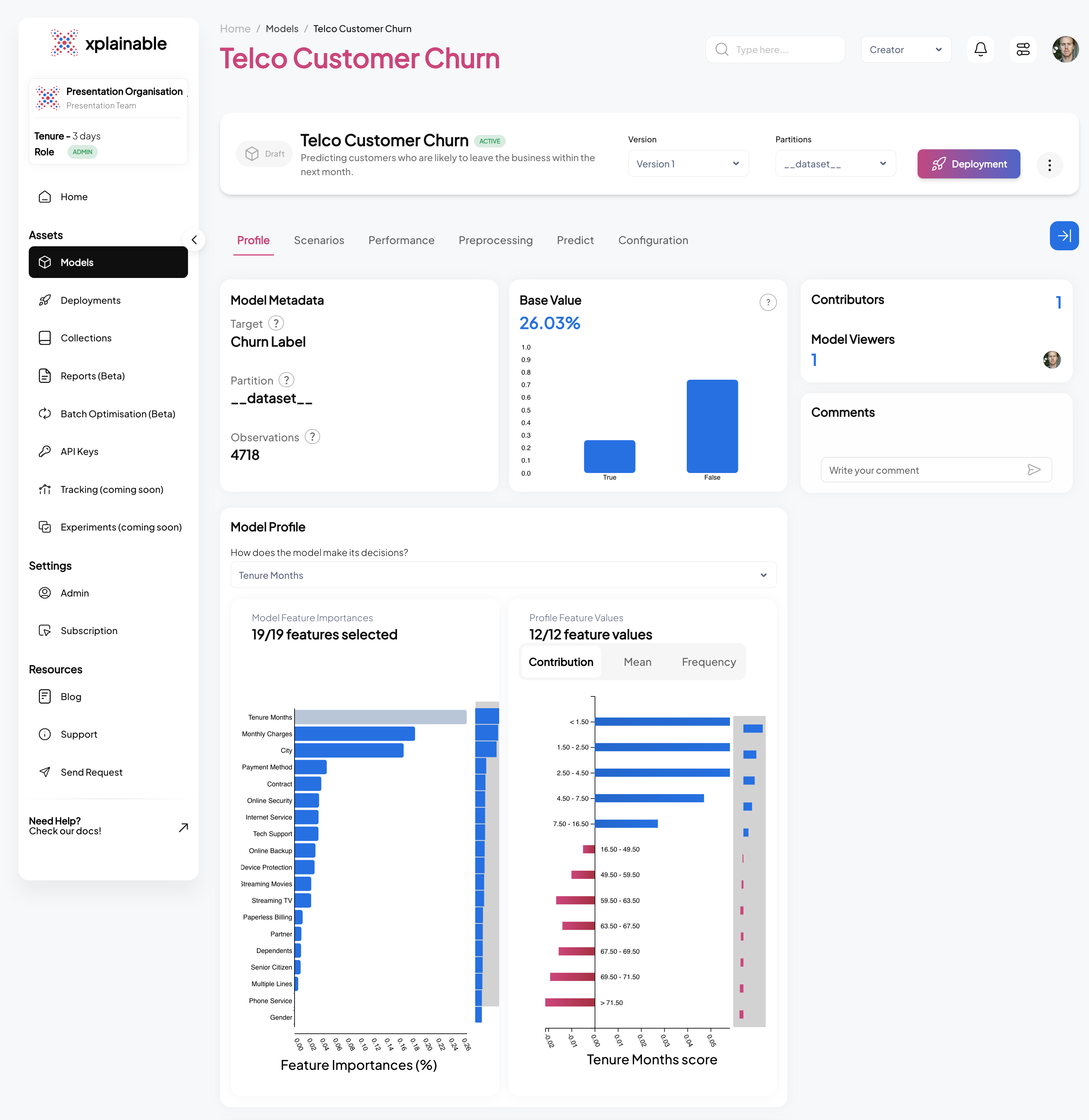
The image displays two graphs related to a churn prediction model.
On the left is the 'Feature Importances' bar chart, which ranks the features by their ability to predict customer churn. 'Tenure Months' has the highest importance, confirming that the length of customer engagement is the most significant indicator of churn likelihood. 'Monthly Charges' and 'Contract' follow, suggesting that financial and contractual commitments are also influential in churn prediction.
The right graph is a 'Contributions' histogram, which quantifies the impact of a specific feature's values on the prediction outcome. The red bars indicate that higher values within the selected feature correspond to a decrease in the likelihood of churn, whereas the green bars show that lower values increase this likelihood.
The placement of 'Gender' at the bottom of the 'Feature Importances' chart conclusively indicates that the model does not consider gender a determinant in predicting churn, thereby ensuring the model's impartiality regarding gender.
5. Model Persisting
In this step, we first create a unique identifier for our churn prediction model using
client.create_model_id. This identifier, shown as model_id, represents the newly
instantiated model which predicts the likelihood of customers leaving within the next
month. Following this, we generate a specific version of the model with
client.create_model_version, passing in our training data. The output version_id
represents this particular iteration of our model, allowing us to track and manage
different versions systematically.
# Create a model
model_id = client.create_model(
    model=model,
    model_name="Lead Scoring",
    model_description="Predicting the likelihood of a lead converting",
    x=X_train,
    y=y_train
)
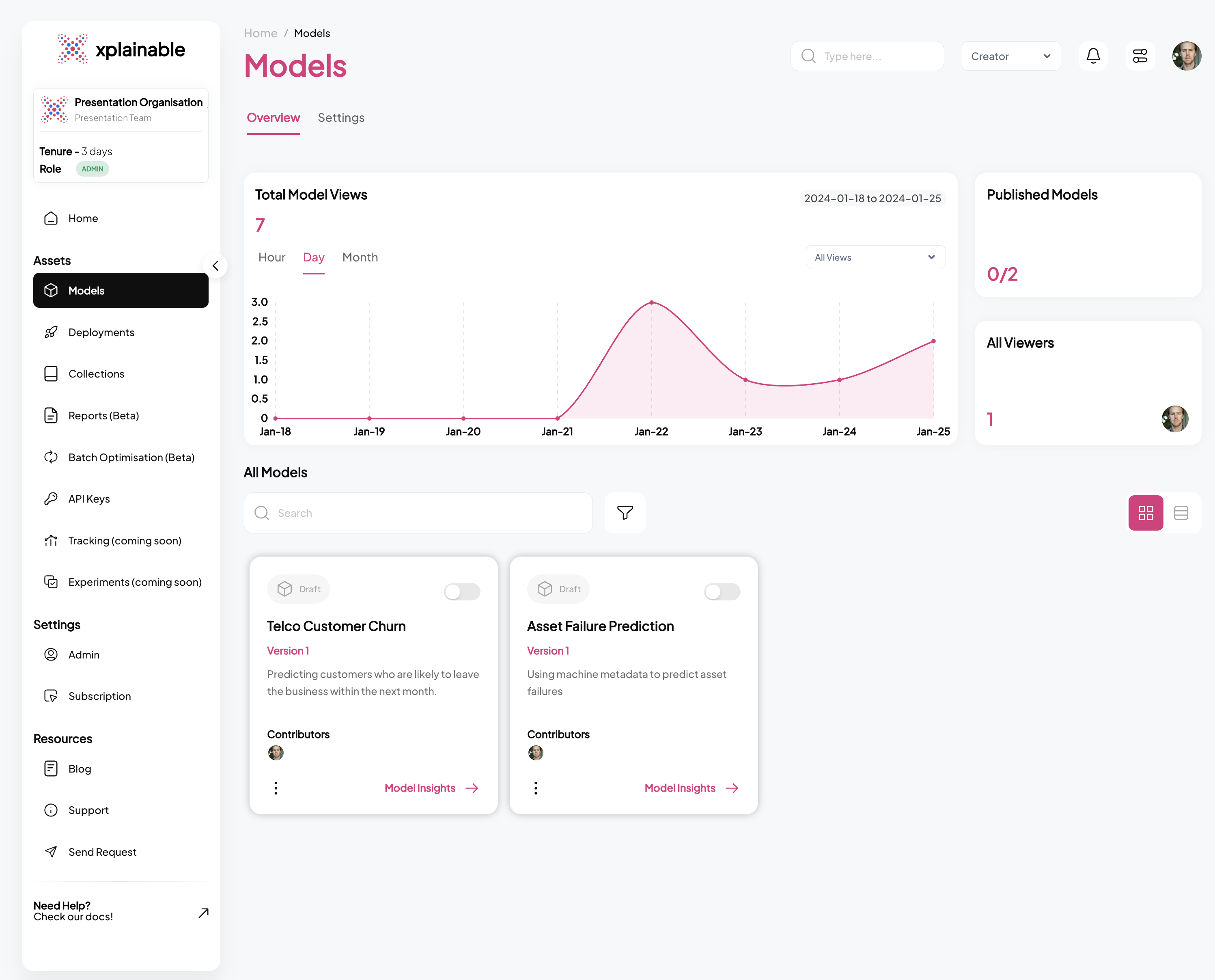
SaaS Models View

SaaS Explainer View

6. Model Deployment
The code block illustrates the deployment of our churn prediction model using the
client.deploy function. The deployment process involves specifying the hostname of
the server where the model will be hosted, as well as the unique model_id and
version_id that we obtained in the previous steps. This step effectively activates the
model's endpoint, allowing it to receive and process prediction requests. The output
confirms the deployment with a deployment_id, indicating the model's current status
as 'inactive', its location, and the endpoint URL where it can be accessed for
xplainable deployments.
deployment = client.deploy(
    model_version_id=model_id["version_id"] #<- Use version id produced above
)
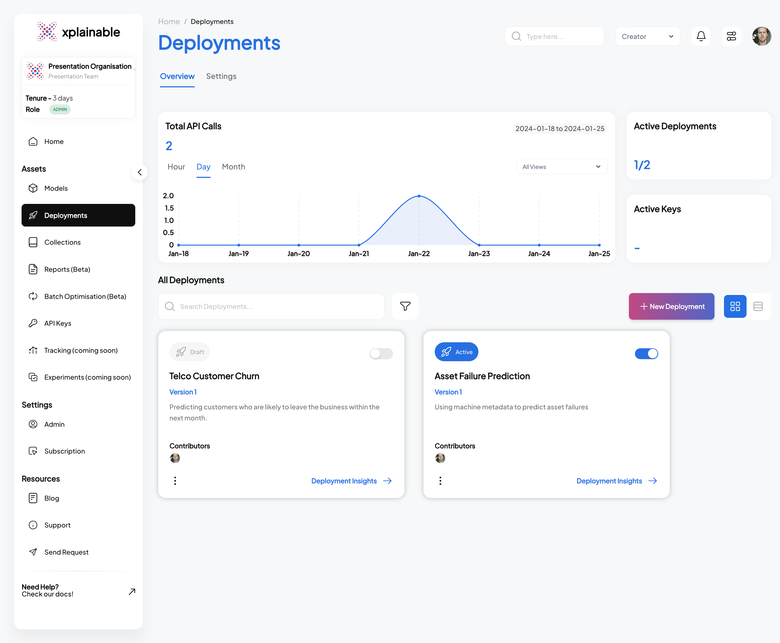
SaaS Deployment View

Testing the Deployment programatically
This section demonstrates the steps taken to programmatically test a deployed model. These steps are essential for validating that the model's deployment is functional and ready to process incoming prediction requests.
- Activating the Deployment: The model deployment is activated using
client.activate_deployment, which changes the deployment status to active, allowing it to accept prediction requests.
client.activate_deployment(deployment['deployment_id'])
- Creating a Deployment Key: A deployment key is generated with
xp.client.generate_deploy_key. This key is required to authenticate and make secure requests to the deployed model.
deploy_key = client.generate_deploy_key(deployment['deployment_id'],'API key for Telco Churn deployment', 7)
- Generating Example Payload: An example payload for a deployment request is
generated by
client.generate_example_deployment_payload. This payload mimics the input data structure the model expects when making predictions.
#Set the option to highlight multiple ways of creating data
option = 2
df_transformed.columns
if option == 1:
    body = client.generate_example_deployment_payload(deployment['deployment_id'])
else:
    body = json.loads(df_transformed.drop(columns=["Converted"]).sample(1).to_json(orient="records"))
    body[0]["Gender"] = None #<- Won't require this line the next release of xplainable
body
- Making a Prediction Request: A POST request is made to the model's prediction endpoint with the example payload. The model processes the input data and returns a prediction response, which includes the predicted class (e.g., 'No' for no churn) and the prediction probabilities for each class.
response = requests.post(
    url="https://inference.xplainable.io/v1/predict",
    headers={'api_key': deploy_key['deploy_key']},
    json=body
)

value = response.json()
value
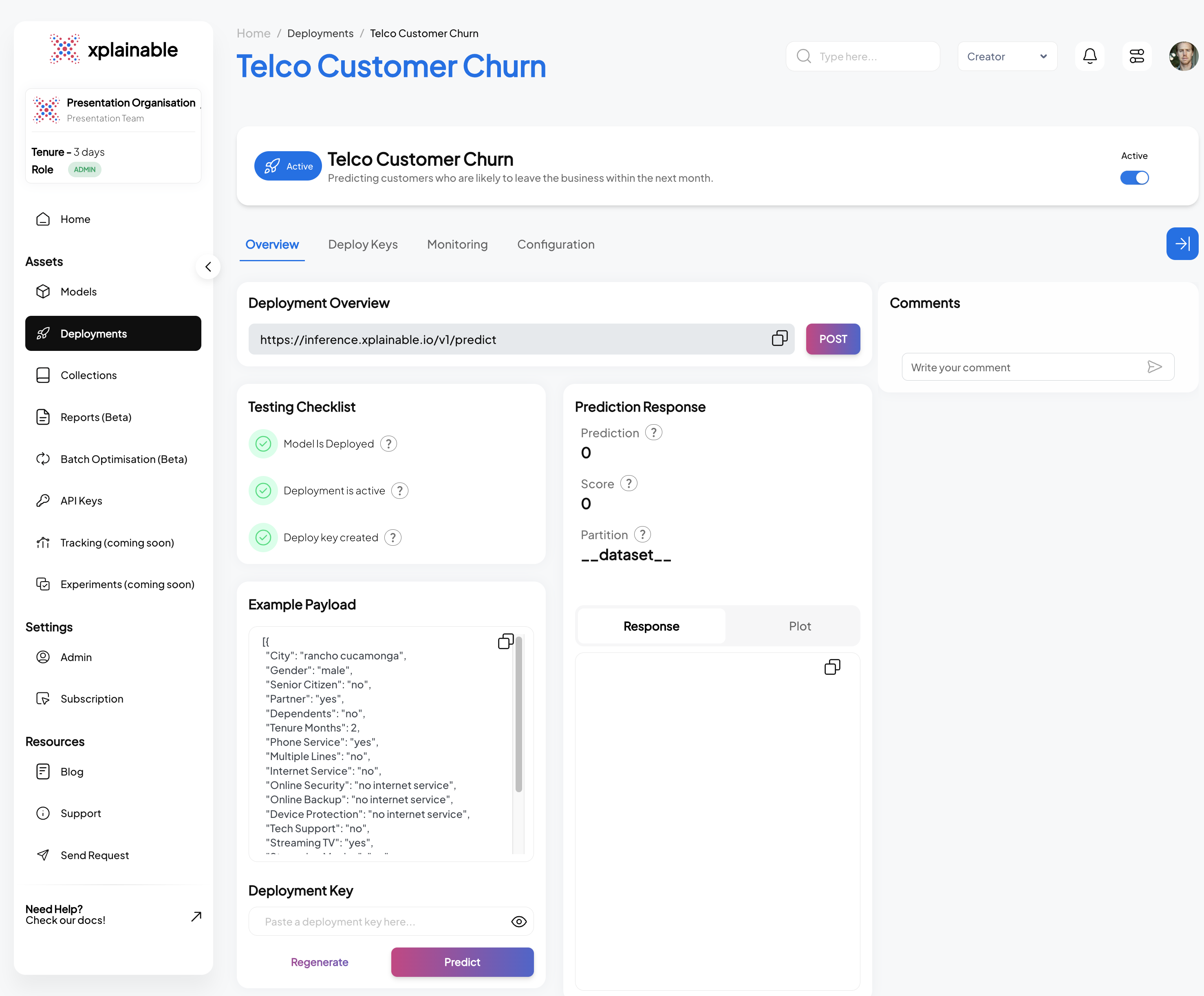
SaaS Deployment Info
The SaaS application interface displayed above mirrors the operations performed programmatically in the earlier steps. It displays a dashboard for managing the 'Telco Customer Churn' model, facilitating a range of actions from deployment to testing, all within a user-friendly web interface. This makes it accessible even to non-technical users who prefer to manage model deployments and monitor performance through a graphical interface rather than code. Features like the deployment checklist, example payload, and prediction response are all integrated into the application, ensuring that users have full control and visibility over the deployment lifecycle and model interactions.

7. Batch Optimisation (Beta)
The concept of Batch Optimization within the Xplainable platform represents a significant leap forward from traditional machine learning approaches. Moving away from the prediction -> monitor model approach, this feature offers a dynamic and cost-effective utilisation of model insights.
This optimisation approach allows for the association of monetary costs with various predictive scores. It provides a detailed understanding of the financial impact of different predictive outcomes. For example, within our Telco model, the choice to provide tech support carries a different cost implication than opting against it, influencing the decision-making process.
Features may be fixed or adjustable to align with business requirements. Certain attributes like 'Senior Citizen', 'Tenure', and 'Monthly Charges' may be set due to regulatory standards or business limitations, ensuring that optimisation adheres to these rules.
Conversely, features such as 'Streaming Movies' or 'Device Protection' are modifiable, enabling the exploration of various combinations to discover the most cost-effective approach. The model could assess if altering the contract type for specific customer segments improves retention without markedly raising costs.
Employing the Xplainable model's output in this manner allows organisations to extend past simple predictions to genuine cost optimisation, facilitating strategic decision-making that evaluates each recommended action not only for its impact on outcomes like churn but also for cost-efficiency. Thus, Xplainable's strategy provides businesses the capability to optimise their resources with foresight rarely seen in traditional machine learning.